pacman::p_load(sf, tmap, tidyverse)Hands-on Exercise 8b: Visualising Geospatial Point Data
1 Learning Outcome
In this hands-on exercise, you will learn how to create a proportional symbol map showing the number of wins by Singapore Pools’ outlets using an R package called tmap:
To import an aspatial data file into R.
To convert it into simple point feature data frame and at the same time, to assign an appropriate projection reference to the newly create simple point feature data frame.
To plot interactive proportional symbol maps.
2 Getting started
3 Geospatial Data Wrangling
3.1 The data
The data set use for this hands-on exercise is called SGPools_svy21. The data is in csv file format.
Figure below shows the first 15 records of SGPools_svy21.csv. It consists of seven columns. The XCOORD and YCOORD columns are the x-coordinates and y-coordinates of SingPools outlets and branches. They are in Singapore SVY21 Projected Coordinates System.
3.2 Data Import and Preparation
The code chunk below uses read_csv() function of readr package to import SGPools_svy21.csv into R as a tibble data frame called sgpools.
sgpools <- read_csv("data/aspatial/SGPools_svy21.csv")After importing the data file into R, it is important for us to examine if the data file has been imported correctly.
The code chunk below shows list() is used to do the job.
list(sgpools) [[1]]
# A tibble: 306 × 7
NAME ADDRESS POSTCODE XCOORD YCOORD `OUTLET TYPE` `Gp1Gp2 Winnings`
<chr> <chr> <dbl> <dbl> <dbl> <chr> <dbl>
1 Livewire (Mar… 2 Bayf… 18972 30842. 29599. Branch 5
2 Livewire (Res… 26 Sen… 98138 26704. 26526. Branch 11
3 SportsBuzz (K… Lotus … 738078 20118. 44888. Branch 0
4 SportsBuzz (P… 1 Sele… 188306 29777. 31382. Branch 44
5 Prime Serango… Blk 54… 552542 32239. 39519. Branch 0
6 Singapore Poo… 1A Woo… 731001 21012. 46987. Branch 3
7 Singapore Poo… Blk 64… 370064 33990. 34356. Branch 17
8 Singapore Poo… Blk 88… 370088 33847. 33976. Branch 16
9 Singapore Poo… Blk 30… 540308 33910. 41275. Branch 21
10 Singapore Poo… Blk 20… 560202 29246. 38943. Branch 25
# ℹ 296 more rowsNotice that the sgpools data in tibble data frame and not the common R data frame.
3.3 Creating a sf data frame from an aspatial data frame
The code chunk below converts sgpools data frame into a simple feature data frame by using st_as_sf() of sf packages
sgpools_sf <- st_as_sf(sgpools,
                       coords = c("XCOORD", "YCOORD"),
                       crs= 3414)
Things to learn from the arguments above:
The coords argument requires you to provide the column name of the x-coordinates first then followed by the column name of the y-coordinates.
The crs argument required you to provide the coordinates system in epsg format. EPSG: 3414 is Singapore SVY21 Projected Coordinate System. You can search for other country’s epsg code by refering to epsg.io.
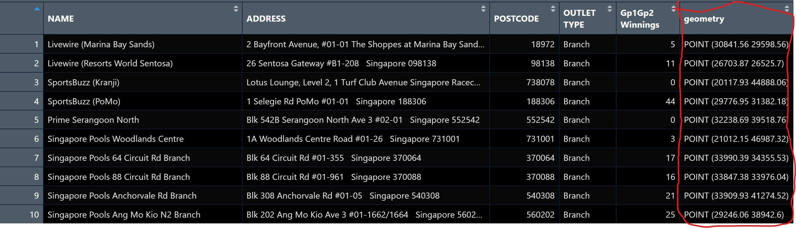
Figure below shows the data table of sgpools_sf. Notice that a new column called geometry has been added into the data frame.
4 Drawing Proportional Symbol Map
The code chunks below are used to create an interactive point symbol map.
tmap_mode("view")
tm_shape(sgpools_sf) +
  tm_bubbles(fill = "red",
           size = 1,
           col = "black",
           lwd = 1)
4.1 Make it proportional
To draw a proportional symbol map, we need to assign a numerical variable to the size visual attribute. The code chunks below show that the variable Gp1Gp2Winnings is assigned to size visual attribute.
tm_shape(sgpools_sf) +
  tm_bubbles(fill = "red",
             size = "Gp1Gp2 Winnings",
             col = "black",
             lwd = 1)
4.2 Lets give it a different colour
The proportional symbol map can be further improved by using the colour visual attribute. In the code chunks below, OUTLET_TYPE variable is used as the colour attribute variable.
tm_shape(sgpools_sf) +
  tm_bubbles(fill = "OUTLET TYPE",
             size = "Gp1Gp2 Winnings",
             col = "black",
             lwd = 1)
4.3 I have a twin brothers :)
An impressive and little-know feature of tmap’s view mode is that it also works with faceted plots. The argument sync in tm_facets() can be used in this case to produce multiple maps with synchronised zoom and pan settings.
tm_shape(sgpools_sf) +
  tm_bubbles(fill = "OUTLET TYPE",
             size = "Gp1Gp2 Winnings",
             col = "black",
             lwd = 1) +
  tm_facets(by= "OUTLET TYPE",
            nrow = 1,
            sync = TRUE)
Before you end the session, it is wiser to switch tmap’s Viewer back to plot mode by using the code chunk below.
tmap_mode("plot")Reference
- Kam, T. S. (2024). Visualising Geospatial Point Data. https://r4va.netlify.app/chap22